Foundations: Tensors & Data
Loading and Preparing Data
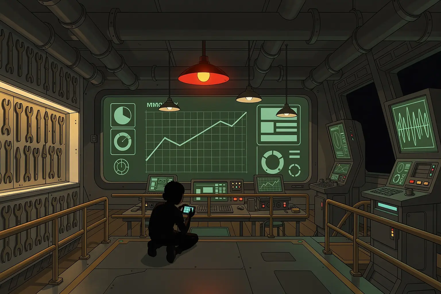
Ensign Demir sets up the data pipeline for the analysis system.

The raw sensor data comes in faster than we can process it in one pass. But this is just infinite scroll, right? Fetch everything once, hold the list, render a window. I pulled the full archive, raw capture blocks and all, into one array overnight.
RangeError: Array buffer allocation failed. Engineering rig, overnight: the loop dies 19,204 readings into a 28,800-reading archive and takes ARIA's diagnostic queue down with it.
The post-mortem arithmetic is short. Each reading drags its 33-second raw capture along: 256 Hz across 64 channels, about two megabytes apiece. Two-thirds of the way through the archive, that is forty gigabytes sitting in one array. Cost of the lesson: a four-hour queue rebuild, logged against Ensign Demir.

Confirmed. Batch processing will allow me to analyze data incrementally while maintaining memory efficiency. I note that I said the same thing about my parsing rules.
What keeps this pipeline alive on real sensor data is where the readings come from. A lazy source reads records on demand. With bounded buffers and correct disposal, memory need not grow with the archive length. .batch(32) sits after that source and sets the model's step size. The model sees 32 readings at a time and asks for the next group when it finishes this one. Demir picked the right analogy and the wrong version of it. A well-built infinite-scroll list keeps the pages it is showing and drops the rest, and a tf.data pipeline does the same with readings.
From Fetch to Feed
You already know half of this pattern. A paginated fetch pulls page 1, hands it off, and never touches page 2 until something asks for it. A tf.data pipeline works the same way, except the thing asking is a model: a generator produces values when the pipeline requests them. Shuffle buffers and prefetching can request records before the model consumes them.
A is one number the model reads about a single example. A is what you want predicted about that example, here a 0 or 1 for whether the reading is worth flagging. The fitDataset training API accepts examples with xs and ys for features and targets. A general tf.data dataset can hold other structures too. Learning from examples that come with their labels attached has a name, , and it is what every model in this course does until module 7, where the model's target is its own input and no human has to label an for it to learn what normal looks like.
Picking which numbers become features is a decision, and on this ship it is already made. A reading's raw capture is 64 channels of samples, about two megabytes per reading, and none of it reaches the model. Three summary values come off each capture instead: amplitude, (a zero-crossing count, not hertz), and phase. The extraction reads a 64-sample window, a quarter second of one channel at 256 Hz, which is a different 64 from the row's 64 channels. Module 5 writes it and then widens the feature set with bins measured over that same window. The classifier you start building in module 2 reads those three, so row.features holds three numbers per reading, not 64 channel values, and xs is three wide. Reading a record still touches its two-megabyte capture block, which is why the source has to hand them over one at a time.
This integration sketch assumes an async readArchivedSample(id) function supplied by your application. It returns one record with features and label; it must not load the entire archive internally. The exercise uses a synchronous in-memory stand-in.
import * as tf from '@tensorflow/tfjs';

// JS: paginated API fetch
// const page = await fetch('/api/data?page=1&limit=32');

// ML: a generator that READS LAZILY, one record per yield.
// Never met "function*"? It declares a GENERATOR: a function that can
// pause at each "yield" and hand out one value, then resume exactly
// where it stopped the next time a value is requested. That pause IS
// the laziness: nothing below the current yield has run yet.
// Each iteration fetches/derives exactly one row; at no point does
// the full archive exist in memory. (If you find yourself declaring
// a giant array inside a generator, you've built eager loading with
// extra steps.)
async function* sensorDataGenerator() {
const TOTAL_READINGS = 28_800;  // 11 days of archive: one reading per 33-second capture

for (let i = 0; i < TOTAL_READINGS; i++) {
  const row = await readArchivedSample(i); // your asynchronous archive reader
  yield {
    xs: tf.tensor(row.features),   // [3]: amplitude, frequency, phase
    ys: tf.tensor([row.label]),
  };
}
}

// Create a dataset pipeline
const dataset = tf.data.generator(sensorDataGenerator)
.shuffle(100)   // shuffle buffer of 100 items: local mixing only
.batch(32);     // group into batches of 32

// Iterate through batches (like paginated API calls)
await dataset.forEachAsync((batch) => {
console.log('Batch shape:', batch.xs.shape); // [32, 3]
});
For independent training examples, shuffle samples before forming . The reason is mechanical. The model adjusts its after every batch, and an archive is stored in the order it was recorded. Without a shuffle each batch is one stretch of one day, so consecutive adjustments all pull the same way. A buffer shuffle chooses from a limited that is refilled as records leave. It does not provide a uniform permutation of the whole archive. Some records can remain in the buffer longer than others, so buffer size is not an exact bound on their age. Here 100 is a demonstration setting.
Sizing the buffer to the whole archive would sample fairly, but a shuffle buffer fills before it yields anything. The first batch would wait for all 28,800 readings, and the pipeline would stop being a stream. So a buffer shuffle is what you are left with when records arrive as a stream you cannot index. This archive can be read by id, so it has a better option: shuffle a list of indices once, up front, and read in that order. That is a full shuffle with no buffer at all, and the split section below builds it.
Why Batching Matters
Batching is virtual-list rendering for model input. A virtual list doesn't render 10,000 DOM nodes at once; it renders a window of visible items. ML models likewise process a window (batch) of data at a time, updating their understanding incrementally.
Memory is only half the reason 32 is the number. The other half is training. The model updates its weights once per batch, using that batch as its estimate of the whole archive: a batch of 1 gives a noisy estimate and a jittery update, and a batch of the full archive gives an exact estimate but one update per pass. Module 3 passes this number to model.fit() and gives the reasoning for a middle value. For now, know that batch size is a knob you set on purpose, not a number the memory limit hands you.
Splitting Without Leaking
Batching decides what the model sees on each step. The split decides what it never sees while training. Get the second one wrong and your validation score is measuring what the model already memorized, not what it learned.
// Hold out the latest 20% of this time-ordered archive for validation
const TOTAL = 28_800;  // the whole archive, the same count the generator walks
const TRAIN_SIZE = Math.floor(TOTAL * 0.8);

// IDs increase with recording time. Assign membership before shuffling.
// Shuffle only the earlier training IDs; validation stays in time order.
const trainIdx = tf.util.createShuffledIndices(TRAIN_SIZE);
const valIdx = Uint32Array.from(
{ length: TOTAL - TRAIN_SIZE }, (_, i) => TRAIN_SIZE + i,
);

async function* splitGenerator(idx: Uint32Array) {
for (const i of idx) {
  const row = await readArchivedSample(i);
  yield { xs: tf.tensor(row.features), ys: tf.tensor([row.label]) };
}
}

const trainData = tf.data.generator(() => splitGenerator(trainIdx)).batch(32);
const valData = tf.data.generator(() => splitGenerator(valIdx)).batch(32);
// Validation contains only later readings. Training order can change
// without moving a reading across the split.
Choose the split for the job the model will do. We want to predict future readings, so validation uses a later period. A classifier that reads one row at a time can still exploit similarities between neighboring rows. Randomly mixing those rows across both sets can make the score too optimistic.
Time order is a starting point. If examples share a capture or overlap in time, keep those groups together and leave a gap at the boundary where needed. Module 6 applies this to overlapping windows. A random split can suit independent examples drawn from the same population as deployment. Whichever rule you choose, assign membership once: separate .shuffle().take() and .shuffle().skip() passes can reshuffle differently and overlap. Fit on training rows only; module 3 adds a final test set that stays out of model selection.
Challenge
Build a lazy pipeline on a 16-row stand-in: generator, shuffle, then batch. This first pipeline demonstrates batching over the whole fixture; it does not train a model. Separately, assign the earlier readings to training and the later ones to validation. Training can shuffle its own rows after that assignment.